Thinking outside inside the Matrix
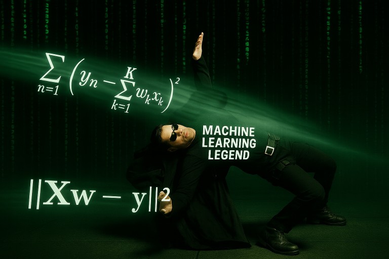
Figure 1: A Machine Learning Legend who can think inside the Matrix and knows when to avoid index notation.
One of the most underrated yet crucial skills to acquire in your machine learning journey is the ability to think and write in terms of matrices, vectors, or sometimes tensors.
What do I even mean by that?
Let’s see a quick example. Below is a quantity expressed in what I call index notation, using sums over indices:
\[\begin{equation} \sum_{n=1}^N \left(y_n - \sum_{k=1}^K w_k x_{n,k}\right)^2 \end{equation}\]And here is the exact same quantity, but this time expressed using matrices and linear algebra operations, in what I call matrix notation:
\[\begin{equation} ||\mathbf{Xw} - \mathbf{y}||_2^2 \end{equation}\](As you may have recognized, this corresponds to the least squares linear regression loss — but this is not important for now).
Why should you care?
Well first, if you’re a student of mine who I practically forced reading this blog post in a somewhat blatant conflict of interest, just know that I mainly use matrix notation during class. So you better get used to it. But, even if you’re not one of my students:
Writing in matrix notation gives you two big advantages over writing in index notation:
-
Speed. The implementation of the former may enable huge speedups in code execution when compared with the latter. And by huge, I mean hundred-plus-fold speedups.
Don’t believe me? You should read part 3 of this article then, you may change your mind.
-
Superpowers. More precisely, the ability to use the unreasonable effectiveness of linear algebra. But asking the linear algebra overlords for help requires speaking their language, namely, that of matrices and matrix operations. This shall be demonstrated in part 2.
So, if you want to go beyond just calling .fit and .predict on your machine learning journey and become a true Machine Learning Legend, thinking in matrices is an essential step forward.
Side note: machine learning, chess, and algebraic notation
One metaphor which I think nicely illustrates my point is chess notation.
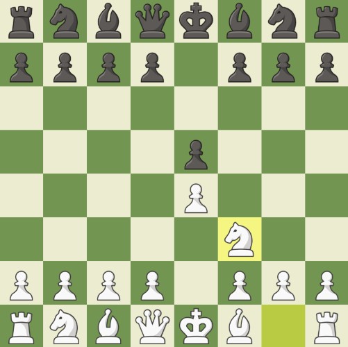
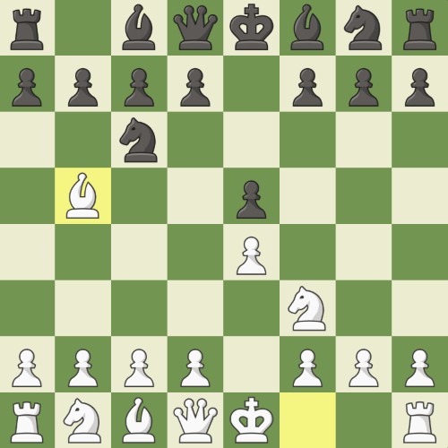
For a beginner, it requires some effort to visualize the actual moves of the pieces on a chessboard from algebraic chess notation such as
1. e4 e5 2. Nf3 Nc6 3. Bb5 a6…
Most of us mere mortals find it much more intuitive to follow chess moves using actual board diagrams.
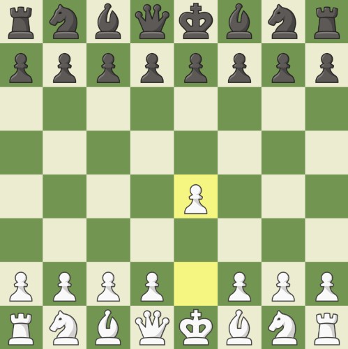
An unremarkable chess game.
However, getting used to going back and forth between the two representations enables keen players to tackle more advanced chess books, ones that don’t spoon-feed you with board diagrams for every move. Ultimately, this is necessary to reach a certain level.
Similarly, writing quantities with sums and indices may be more intuitive to many people* at first, particularly people coming from a Computer Science background, who tend to think in terms of for loops. But being able to effortlessly translate index notation to matrix operations and vice versa is ultimately necessary to go beyond surface-level understanding of machine learning.
*Myself included. I personally only started actively developing this skill during my PhD, after a MSc in machine learning and a couple of years of professional experience as a data scientist. So whatever your current level of machine learning proficiency, there is nothing to be ashamed of. It’s always better to start now than never.
The objective of this article is to let you take that initial step, and make you a seasoned machine learning walker who can effortlessly tread through the hills of more advanced linear algebra. In particular, throughout other posts in this blog, I mostly assume you are well-versed in this exercise.
But I promise, with enough practice, it’s really not that difficult. So let’s get started!
A first example: linear regression
Basic “naive” formulation
To understand how all of this works, let’s start with a very basic example: (multivariate) linear regression.
Note: my goal here is to use linear regression as an example, not explain how it works. I assume readers are already somehow familiar with basic machine learning concepts, including linear regression.
Let’s say we have $K$ input variables $x_1, x_2, \dots, x_K$ — for instance, the square footage of an apartment $x_1$, its number of bedrooms $x_2$ and distance to city center $x_3$, in which case $K=3$. We want to estimate the price of this apartment. Our estimation or prediction $\hat{y}$ will be a linear combination of the inputs:
\[\begin{align*} \hat{y} &= w_1 \cdot x_1 + w_2 \cdot x_2 + \dots + w_K \cdot x_K \\ &= \sum_{k=1}^K w_k x_k \end{align*}\]where $w_1, \dots, w_K$ are the parameters or weights of the model.
In standard linear regression, the parameters are learned on a bunch of labeled training examples to minimize some training error. So let’s say we have a total of $N$ different samples: for instance, we may have access to the data (square footage, bedrooms etc.) of $N=100$ apartments, along with their corresponding actual selling prices $y_1, y_2, \dots, y_N$. For apartment number $n$, we consider features $x_{n,1}, \dots, x_{n,K}$, where $x_{n,k}$ is the $k^\text{th}$ feature of the $n^\text{th}$ apartment. The prediction is then
\[\hat{y}_n = \sum_{k=1}^K w_k x_{n,k}\]In the usual least squares formulation of linear regression, we want to find parameters $w_1, \dots, w_K$ which minimize the squared prediction errors on the training dataset. For apartment number $n$, the squared difference between prediction $\hat{y}_n$ and the actual price $y_n$ is \((\hat{y}_n - y_n)^2\). Thus,
The error or loss $\mathcal{L}$ for the whole training dataset is:
\[\begin{align*} \mathcal{L} &= \sum_{n=1}^N (\hat{y}_n - y_n)^2 \\ &= \sum_{n=1}^N \left(\left(\sum_{k=1}^K w_k x_{n,k} \right) - y_n\right)^2 \end{align*}\]OK, looks easy enough.
So then, please remind me: why would there by any issue with this notation? Why should we prefer matrix notation such as
\[||\mathbf{Xw} - \mathbf{y}||_2^2\](which we will derive shortly in part 2) over the previous nice, easy-to-implement double sum with index notation from Equation (1)?
Well, as I said, for two reasons: speed, and the ability to use results from linear algebra. I promise, I will make these two advantages as explicit as I possibly can in very short order. But for now, let’s focus on how we can transform Equation (1) into Equation (2), so that we can compare the two approaches.
The Golden Rule of matrix thinking
Below is the central idea of matrix thinking, which I will refer to as the Golden Rule.
I don’t think that’s a real name, I just made it up for dramatic effect. But it’s a neat name to really drive my point across.
Please note: the latter notation $\mathbf{a}^\top\mathbf{b}$ is the one I use most commonly to denote a dot product.
Where does this notation come from?
The notation $\mathbf{a}^\top\mathbf{b}$ implicitly turns the column vector \(\mathbf{a} = \begin{pmatrix} a_1 \\ a_2 \\ \vdots \\ a_K \end{pmatrix} \in \mathbb{R}^K\) into a row vector $\mathbf{a}^\top = \begin{pmatrix} a_1 ~ a_2 ~ \dots ~ a_K \end{pmatrix}$ with the transpose operation $(\cdot)^\top$.
Vector $\mathbf{a}$ can also be viewed as a matrix with $K$ rows and $1$ column, so $\mathbf{a}^\top$ can be viewed as a matrix of size $1 \times K$.
$\mathbf{a}^\top$ is then matrix-multiplied with the column vector \(\mathbf{b} = \begin{pmatrix} b_1 \\ b_2 \\ \vdots \\ b_K \end{pmatrix} \in \mathbb{R}^K\), which is also a matrix of size $K \times 1$. The matrix multiplication $\cdot$ of $\mathbf{a}^\top \in \mathbb{R}^{1 \times K}$ with $\mathbf{b} \in \mathbb{R}^{K \times 1}$ results in a matrix $\mathbf{a}^\top \cdot \mathbf{b}$ of size $1 \times 1$, implicitly cast as a scalar $\in \mathbb{R}$.
I typically use this type of notation a lot, as this is quite convenient.
Depending on your background, this so-called “Golden Rule” may seem painfully obvious. But, similarly to the pigeonhole principle, stupidly obvious statements can sometimes lead to interesting and far from obvious results.
Applying the Golden Rule to linear regression
Let’s see how we can apply the Golden Rule to get rid of the sums and indices in Equation (3) and transform it into Equation (4).
First sum over $k$
From our example from earlier: for apartment/sample number $n$, the predicted price/target is given by
\[\hat{y}_n = \sum_{k=1}^K w_k x_{n,k}\]Using the Golden Rule™, this can be rewritten as
\[\hat{y}_n = \mathbf{w}^\top \mathbf{x}_n\]where \(\mathbf{w} = \begin{pmatrix} w_1 \\ \vdots \\ w_K \end{pmatrix} \in \mathbb{R}^K\) represents the $K$ parameters of the linear model as a column vector, and \(\mathbf{x}_n = \begin{pmatrix} x_{n,1} \\ \vdots \\ x_{n,K} \end{pmatrix}\in \mathbb{R}^K\) corresponds to the $K$ input variables of the $n^\text{th}$ sample, also stacked in a vector.
We can go a step further: if we define a vector $\hat{\mathbf{y}} \in \mathbb{R}^N$ whose elements are \(\begin{pmatrix} \hat{y}_1 \\ \vdots \\ \hat{y}_N \end{pmatrix}\), we have
\[\hat{\mathbf{y}} = \begin{pmatrix} \mathbf{x}_1^\top\mathbf{w} \\ \vdots \\ \mathbf{x}_N^\top\mathbf{w} \end{pmatrix}\]Notice anything? A vector whose elements are given by different linear combinations of the same vector $\mathbf{w}$ with different coefficients $\mathbf{x}_1, \dots, \mathbf{x}_N$ is pretty much the definition of a matrix-vector multiplication.
Thus, we can “stack” all the $N$ sample vectors $\mathbf{x}_1, \dots, \mathbf{x}_N$ into a matrix with $N$ rows and $K$ columns:
\[\mathbf{X} = \begin{pmatrix} x_{1,1} & x_{1,2} & \dots & x_{1,k} & \dots & x_{1,K} \\ x_{2,1} & x_{2,2} & \dots & x_{2,k} & \dots & x_{2,K} \\ \vdots & \vdots & & \vdots & & \vdots \\ x_{n,1} & x_{n,2} & \dots & x_{n,k} & \dots & x_{n,K} \\ \vdots & \vdots & & \vdots & & \vdots \\ x_{N,1} & x_{N,2} & \dots & x_{N,k} & \dots & x_{N,K} \end{pmatrix} = \begin{pmatrix} \mathbf{x}_1^\top \\ \vdots \\ \mathbf{x}_N^\top \end{pmatrix} = \begin{pmatrix} \mathbf{x}_1 & \dots & \mathbf{x}_N \end{pmatrix}^\top \in \mathbb{R}^{N \times K}\]A quick word on notation
In general throughout this blog, matrices are denoted by uppercase bold letters (e.g. $\mathbf{X}$), vectors by lowercase bold letters (e.g. $\mathbf{x}$), and scalars by non-bold letters (e.g. $k$, $N$ or $x_{n,k}$). This is a fairly common and quite useful convention, as this makes the nature of each variable/object much clearer in equations.
Using this convention, the matrix \(\mathbf{X} = \begin{pmatrix} x_{1,1} & \dots & x_{1,K} \\ \vdots & \ddots & \vdots \\ x_{N,1} & \dots & x_{N,K} \end{pmatrix} \in \mathbb{R}^{N \times K}\) can also be more succinctly expressed as \(\mathbf{X} = \begin{pmatrix} \mathbf{x}_1^\top \\ \vdots \\ \mathbf{x}_N^\top \end{pmatrix}\) (column vectors $\mathbf{x}_n \in \mathbb{R}^{K}$ are transposed to row vectors and then vertically stacked) or as $\mathbf{X} = \begin{pmatrix} \mathbf{x}_1 ~\dots ~ \mathbf{x}_N \end{pmatrix}^\top$ (column vectors $\mathbf{x}_n$ are horizontally aligned next to each other, and the resulting $K \times N$ matrix is transposed to obtain the desired $N \times K$ matrix).
And finally, we can directly express $\hat{\mathbf{y}}$ as the matrix-vector multiplication of $\mathbf{X}$ and $\mathbf{w}$:
\[\begin{equation} \hat{\mathbf{y}} = \mathbf{Xw} \in \mathbb{R}^N \end{equation}\]We can double-check that \(\hat{y}_n = \sum_{k=1}^K x_{n,k} w_k\) indeed corresponds to the formula for the $n^\text{th}$ row of a matrix-vector multiplication between a matrix $\mathbf{X}$ (whose element at row $n$ and column $k$ is given by $x_{n,k}$) and the vector $\mathbf{w}$ (whose $k^\text{th}$ element is $w_k$).
Vectors as operators on matrices
In general, for expressions of the form $\mathbf{Ab}$, we tend to think of matrix $\mathbf{A}$ as a linear operator, which applies a different linear map (defined by $\mathbf{a}_k$ the $k^\text{th}$ row of $\mathbf{A}$) to every element $b_k$ of vector $\mathbf{b}$, such that element $k$ of vector $\mathbf{Ab}$ is given by \((\mathbf{Ab})_k = \mathbf{a}_k^\top\mathbf{b} = \sum_i a_{k,i} b_i\)
In our specific case here, we would be tempted to say that the opposite is happening: the coefficients $\mathbf{w}$ of the linear regression define a linear map that is applied to every sample $\mathbf{x}_n$ to obtain the prediction $\hat{y}_n = \mathbf{w}^\top \mathbf{x}_n$. In my explanation earlier, I stated instead that $\mathbf{x}_n$ is a linear map that is applied to $\mathbf{w}$ to obtain row $\hat{y}_n$, which may sound a bit weird.
However, since $\mathbf{w}^\top \mathbf{x}_n = \mathbf{x}_n^\top\mathbf{w}$, the two formulations are equivalent in this situation, and the latter makes the matrix-vector multiplication relationship between $\hat{\mathbf{y}}$, $\mathbf{X}$ and $\mathbf{w}$ a bit more evident IMHO.
Thinking in terms of tensors with covariant and contravariant coordinates may sometimes be helpful to keep ideas clear about what is an operand and what is an operator. A blog post on this topic should be coming soon.
However, I would advise that you don’t explore this until you are already quite familiar with matrix notation. A good test of readiness may be your ability to effortlessly solve the exercises included at the end of this article.
A piece of advice that will recur frequently throughout this article: it is pretty much always a good idea to quickly check that the dimensions of our mathematical objects (matrices, vectors, and others) are consistent.
As an example, in Equation (3), $\mathbf{X} \in \mathbb{R}^{N \times K}$ and $\mathbf{w} \in \mathbb{R}^{K}$, so $\mathbf{Xw} \in \mathbb{R}^{N}$. We were supposed to have $\hat{\mathbf{y}} \in \mathbb{R}^{N}$, so all is good. ✅
Second sum over $n$
OK, we got rid of one of the sums in Equation (3), the one over $k$. What about the second one, the one over $n$?
\[\sum_{n=1}^N (\hat{y}_n - y_n)^2\]Is this a sum of products?
Well, yes: $(\hat{y}_n - y_n)^2 = (\hat{y}_n - y_n)(\hat{y}_n - y_n)$ (duh!)
So writing e.g. $\mathbf{z} = \hat{\mathbf{y}} - \mathbf{y}$ (i.e. $z_n = \hat{y}_n - y_n ~~ \forall n$), we can use the same idea as before:
\[\sum_{n=1}^N (\hat{y}_n - y_n)^2 = \sum_{n=1}^N z_n z_n = \mathbf{z}^\top\mathbf{z} = (\hat{\mathbf{y}}-\mathbf{y})^\top(\hat{\mathbf{y}}-\mathbf{y})\]In general, instead of \(\mathbf{z}^\top\mathbf{z}\), we tend to write \(||\mathbf{z}||_2^2\), but the idea is the same.
🧮 Why are they equal?
By definition \(||\mathbf{z}||_2 = \sqrt{\sum_{k=1}^K z_k^2}\)
So \(||\mathbf{z}||_2^2 = \sum_{k=1}^K z_k^2\)
Thus,
\[\sum_{n=1}^N (\hat{y}_n - y_n)^2 = ||\hat{\mathbf{y}} - \mathbf{y}||_2^2\]And finally, since $\hat{\mathbf{y}} = \mathbf{Xw}$, we can write:
Again, depending on your background, what we just did may look either super obvious or needlessly complicated. But again, doing this can be a really really powerful tool when used correctly in the right context, because this then enables us to leverage the 🌈full power of linear algebra🌟.
Making use of our newly unlocked power

Figure 2: A poorly disguised Sylvester equation about to be annihilated by the full power of linear algebra (exercise 9).
What do I mean by this? Well, recall that in linear regression, we want to find weights $w_1, \dots, w_K$ that minimize our loss $\mathcal{L}$ (the sum of squared residues) on our training dataset. Directly minimizing our cost function written in index notation with respect to its parameters does not seem to be an easy problem, at least to me:
\[\underset{w_1, \dots, w_K}{\text{minimize}} \sum_{n=1}^N (y_n - \sum_{k=1}^K w_k x_{n,k})^2\]How about this exact same problem, but formulated with matrix notation?
\[\underset{\mathbf{w}}{\text{minimize}} ~ ||\mathbf{Xw} - \mathbf{y}||_2^2\]Turns out, problems of the form \(\underset{\mathbf{w}}{\text{minimize}} ~ ||\mathbf{Aw} - \mathbf{b}||_2^2\) are super standard problems with a well-known solution, in this case:
\[\mathbf{w} = \mathbf{X}^\dagger\mathbf{y}\]where $\mathbf{X}^\dagger = (\mathbf{X}^\top\mathbf{X})^{-1}\mathbf{X}^\top$ is called the pseudo-inverse of $\mathbf{X}$.
(You may also read this other post for more details about where this formula comes from. However, the post assumes that you are already reasonably familiar with matrix notation, so I would advise you practice with the exercises below first).
So this is one possible implementation of linear regression:
def get_linear_regression_coefficients(samples: np.ndarray, labels: np.ndarray) -> np.ndarray:
    """
    Given training matrix of samples of shape (N,K) and vector of labels of shape (N,),
    return the coefficients of the least squares linear regression model
    as an array of shape (K,).
    """
    return np.linalg.inv(samples.T @ samples) @ samples.T @ labels
Boom. We just solved linear regression in one line. No need for gradient descent or any of that: we can get the optimal parameters of our model in literally one line of code.
Other gifts from the linear algebra overlords
Important preamble: This part provides additional examples of problems that seem hard when written in index notation, but become fairly easy when written in matrix notation. This section moves at a rather brisk pace: its purpose is more to show what you can do once you get familiar with matrix notation and matrix calculus, rather than to really explain how to get there. So if you’re reading this article for the first time, feel free to skip ahead to the next section for now. It is probably more relevant to do some practice exercises (graciously provided at the end of the article) first, before trying to read this section for the first time.
I'm not afraid, show me your full power!
OK, so, is writing in matrix notation mostly useful for solving one problem, namely least squares linear regression?
Well, of course not. Did you really think I would make an entire post just to talk about linear regression? I mean, yeah, I absolutely could have done that, fair enough. But no, in this case I didn’t.
Getting back to our main topic: writing in matrices really is a ubiquitous tool, especially when combined with other tools like matrix calculus.
Principal Component Analysis
Let’s quickly consider another example: Principal Component Analysis (a.k.a. PCA for family and friends). In PCA, given $N$ unlabeled training samples $(\mathbf{x}_1, \dots, \mathbf{x}_N)^\top$ in $K$ dimensions, we want to find a direction $\mathbf{w} \in \mathbb{R}^K$ (a unit-norm vector) along which variance is maximized when points are projected onto this direction.
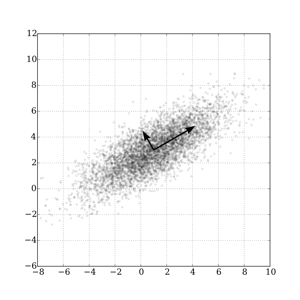
Illustration of the principal components of a 2-dimensional multivariate Gaussian distribution, from Wikipedia.
The norm of the projection of vector $\mathbf{x}_n$ along vector $\mathbf{w}$ is given by $\mathbf{x}_n^\top\mathbf{w}$ when \(||\mathbf{w}||_2 = 1\) (cf. exercise 4 below), so assuming points are centered, we want to solve:
\[\underset{\mathbf{w}}{\text{maximize }} \left(\frac{1}{N}\right) \sum_{n=1}^N (\mathbf{x}_n^\top\mathbf{w})^2 \quad \text{such that } ||\mathbf{w}||_2=1\]If we insist on writing this in full index notation, this is our problem:
\[\underset{w_1, \dots, w_K}{\text{maximize }} \sum_{n=1}^N \left( \sum_{k=1}^K x_{n,k}w_k\right)^2 \quad \text{s.t. } \sqrt{\sum_{k=1}^K w_k^2} = 1\]Again, this problem does not seem so easy at first glance.
But wait… A bunch of elements with the $n^\text{th}$ element being equal to $\mathbf{x}_n^\top\mathbf{w}$? We’ve seen that already, that’s $\mathbf{Xw}$. The sum of the squares of these elements? That’s the $\ell 2$ norm of this vector. The constraint on the norm of $\mathbf{w}$ is slightly trickier to deal with, but can be tackled with a Lagrange multiplier $\lambda$ (maybe I’ll write an article on this topic some day).
So in matrix form, our problem can be written as
\[\underset{\mathbf{w}}{\text{maximize }} ||\mathbf{Xw}||_2^2 + \lambda(1-||\mathbf{w}||_2^2)\]A trivial application of matrix calculus (exercise 8 of referenced blog post) yields that the quantity above is maximized if
\[\mathbf{X}^\top\mathbf{Xw} = \lambda \mathbf{w}\]i.e. if $\mathbf{w}$ is an eigenvector of the covariance matrix $\mathbf{X}^\top\mathbf{X}$.
Wanna try getting this result without explicitly writing $\mathbf{X}$ as matrix? Good luck with that.
And we could even continue further with PCA: once we have computed the first $C$ principal components $\mathbf{P} = (\mathbf{p}_1, \dots, \mathbf{p}_C)^\top \in \mathbb{R}^{C \times K}$ as the first $C$ eigenvectors of the covariance matrix $\mathbf{X}^\top\mathbf{X} \in \mathbb{R}^{K \times K}$ (one line of code using NumPy), the transform operation is $\mathbf{Z} = \mathbf{XP}^\top$. The inverse transform operation is $\hat{\mathbf{X}} = \mathbf{ZP}$.
So there you have it: once you speak the language of the gods (i.e. the language of matrices, in case you haven’t been following at all), deriving PCA is a few lines of calculations. A working implementation is a few lines of code.
Sylvester equations
OK, one last (optional) example to really hammer it in.
Given $3 \times N \times N$ values $a_{m,n}, b_{m,n}, c_{m,n}$ for $(m,n) \in \{1, \dots, N \}^2$, find $N \times N$ values $x_{m,n}$ such that
\[\sum_k (a_{m,k}x_{k,n} + b_{k,n}x_{m,k} - \frac{1}{N^2}c_{m,n}) = 0 \quad \forall m,n\]Finished yet? No? Yeah, I didn’t think so.
Let’s rewrite it in matrix form (exercise 9):
\[\mathbf{AX} + \mathbf{XB} = \mathbf{C}\]Boom! That’s a Sylvester equation. It’s as good as solved.
Now, I need to refrain from going on and on about how the exact same trick can be applied to low-rank matrix factorization for recommendation systems, to Support Vector Machines, to everything related to deep learning… I think you get my point.
The point.
Hopefully, I managed to convince you that many machine learning methods can only be truly understood through the lens of linear algebra.
But, what is really the point of all of this? Is being able to derive the analytical solution to least squares linear regression or similar problems of any practical use? After all, there are literally dozens of libraries that can do this automatically for us.
Well, I’m glad you asked!
First, I 100% guarantee that someone mindlessly .fit.predicting (yes, that’s a word now) their way to predictions using existing implementations without understanding how the underlying algorithm works is bound to make some dumb mistakes sooner or later. I could tell you quite a few horror stories on this topic, and I probably will in a future blog post. So in general, the more you know, the less likely you are to do something stupid.
Second, truly mastering the basics is a prerequisite to identifying situations where the same ideas can be applied to obtain non-trivial results. After all, this is what this blog is supposed to be about — and this should hopefully be illustrated soon enough with real case studies on e.g. 3D facial shape estimation from photos, or internal bone shape estimation from 3D skin surface mesh. So stay tuned!
And of course, mastering the basics is also a prerequisite to work on cutting-edge topics. Mastering PCA is a first step in mastering auto-encoders. Auto-encoders lead to VAEs. VAEs lead to diffusion models, diffusion models lead to the dark side image generation models — which are great to generate awesome illustrations for ridiculously technical blog posts.
And guess what? Being really comfortable with matrix notation can be of huge help when learning about these topics. So let’s continue!
The case for speed
In addition to the ability to easily solve seemingly hard problems, I mentioned that a second big advantage to writing everything in matrix/vector format is speed of execution.
So, let’s do a very quick test that should hopefully help me convert any remaining non-believer.
Implementation with index notation
Let’s first create a reasonably large dummy dataset for test purposes using NumPy.
# Let's define some randomly generated test data
import numpy as np
np.random.seed(42)

N, K = 50000, 1000 # number of samples N and dimension K of feature space
X = np.random.randn(N, K) # our feature matrix, shape (N,K)
y = np.random.randn(N) # our target vector, shape (N,)
w = np.random.randn(K) # some weights for our linear model, shape (K,)
Let’s try a first approach where we compute the error $\mathcal{L}$ on this fairly large dataset using sums and for loops, based on the index notation:
\[\mathcal{L} = \sum_{n=1}^N (\sum_{k=1}^K w_k x_{n,k} - y_n)^2\]def make_prediction(weights: list, sample: list) -> float:
"""Make one prediction as a linear combination of inputs and weights."""
total = 0
for wi, xi in zip(weights, sample):
total += wi * xi
return total
def compute_error(weights: list[float], samples: list[list[float]], targets: list[float]) -> float:
"""Compute the sum of the squared error between the prediction and the target on the full dataset."""
total_error = 0
for xn, yn in zip(samples, targets):
prediction = make_prediction(weights, xn)
error = prediction - yn
total_error += error ** 2
return total_error
Running this:
print(compute_error(w, X, y))
takes about 3.4 seconds on my computer.
Notice that there is nothing particularly wrong with this code, it is a mostly straightforward Python implementation of the formula above.
Implementation with matrix notation
Now let’s compute the exact same thing, this time using linear algebra operations from NumPy to implement the loss directly from matrix notation:
\[\mathcal{L} = ||\mathbf{Xw} - \mathbf{y}||_2^2\]def compute_error_with_linear_algebra(weights: np.ndarray, samples: np.ndarray, targets: np.ndarray) -> float:
"""Same as above, this time using the linear algebra formulation."""
return np.linalg.norm(X @ w - y) ** 2
print(compute_error_with_linear_algebra(w, X, y))
The numerical result we obtain is exactly the same, but this time the code ran in…
🥁
🥁
🥁
22 milliseconds. That is more than 100 times faster!
Why is it so fast?
Very briefly: Python is an interpreted language that is quite slow overall, whereas there are hyper-optimised linear algebra libraries (on top of which Python wrappers such as NumPy are built) which make smart use of CPU caches and specific CPU instructions to do matrix multiplication very, very efficiently. Hence the performance difference when we use the latter, even when they are called from our slow Python code.
And we did not even go into GPU territory! Writing native, efficient CUDA code is a huge pain in the gluteus maximus, but simply writing everything in terms of matrices/tensors makes it super easy to run our pipeline with Pytorch or other specialised frameworks that do all the heavy-lifting for us.
Also, it is noteworthy that we are not even solving the linear regression problem yet. We were merely computing the cost. If we instead compare our analytical solution from earlier with a multistep gradient descent solver with numerical gradient estimation implemented using sums over indices, we’re not talking about a 100-fold performance gain anymore. More likely a 10000-fold. To emphasize, this is not an instance where I’m deliberately exaggerating to prove a point: I quite literally mean that the latter approach would converge approximately 10,000 times more slowly.
Don’t believe me? I am currently in the process of writing a bonus part to this (already way too long) blog post, in which I should hopefully be able to demonstrate a billion-fold speed-up thanks to the power of matrix notation. So stay tuned!
OK, we are running short on time, so we only have time for one more question from the imaginary audience. Umm, you there, please go ahead.
“One toy example is nice, but my question is: does this translate to actual improvements in practice?”
Yes. Yes yes yes. Oh yes, trust me, it does. There were several occasions where I was able to achieve similar or even higher performance improvements to existing code. And let me tell you, achieving a 1000-fold speedup in production code is a great way to come across as a true Machine Learning Legend™.
Practice time!
Congrats on following so far! Hang in there, you only have a few steps left before completing your initiation to the divine language of matrix notation. But first, I have some good news and some bad news.
The bad news: seamlessly translating sums and loops to vector and matrix operations or vice versa is (generally) not an innate ability — at least it wasn’t for me. As with everything worth doing, it takes some practice to get comfortable in this exercise.
The good news: practice is what this section is for! For each of the examples below, try to either write it in matrix notation if it is written with sums over indices, or vice versa. As a bonus, you can also try to write the corresponding code with a linear algebra library such as NumPy.
You may look at the solution to the first exercise (which is a really basic example) to clarify what is being asked if you want. But ideally, you should try to do the others yourself.
Hints: some of these exercises may require the use of:
- The $\ell 1$ norm \(||\cdot||_1\): for vector $\mathbf{a} \in \mathbb{R}^K$,
- The element-wise or Hadamard product $\odot$: for matrices $\mathbf{A}$ and $\mathbf{B}$ with compatible dimensions:
- The all-$0$ or all-$1$ vectors $\boldsymbol{0}$ or $\boldsymbol{1}$:
A final piece of advice: before diving headfirst into the calculations, ask yourself: what is the nature of the result and the different operands involved? Are they scalars, vectors, matrices? Are their dimensions compatible?
All right! I have been doing all the work so far; now it’s your turn!
Exercise 0 (demo)
\[\sum_j a_{i,j} b_j\]Solution
There are two indices $i$ and $j$ for object $a$, so it seems to be a matrix, which we can write $\mathbf{A}$ (cf. the quick note on notation earlier). Assuming $i$ ranges from $1$ to some integer $I$, and $j$ from $1$ to $J$, $\mathbf{A}$ is of size $I \times J$, i.e. $\mathbf{A} \in \mathbb{R}^{I \times J}$.
Similarly, there is only one index $j$ for $b$, so it is probably a vector, which we can write $\mathbf{b} \in \mathbb{R}^J$.
We are summing over index $j$, multiplying $a_{i,j}$ with $b_j$. This is a dot product between $\mathbf{a}_i$, the $i^\text{th}$ row of $\mathbf{A}$, and $\mathbf{b}$. Since we are not summing over $i$, we can assume that we perform this operation for every $i$ in ${1, \dots, I}$, resulting in a vector of size $I$.
Performing $I$ distinct dot products, each defined by the row of a matrix, is the definition of a matrix-vector multiplication. So, we can rewrite this as
\[\mathbf{A}\mathbf{b} \in \mathbb{R}^I, \quad \text{with } \mathbf{A} \in \mathbb{R}^{I \times J} \text{ and } \mathbf{b} \in \mathbb{R}^J\]NumPy implementation: assuming variables A and b have been previously defined, for example with:
# Initialize random matrix and vector
I, J = 3, 4
A = np.random.randn(I,J)
b = np.random.randn(J)
the operation above can be written as:
# Perform matrix-vector multiplication
A @ b
# or equivalently: np.dot(A, b), or A.dot(b)
Show exercises
Other practice exercises
Exercise 1
\[\sum_i (a_{i} - b_i) b_i\]Solution
$a$ and $b$ have one shared index $i$, so they seem to be vectors with the same dimension. Assuming again that $i$ ranges from $1$ to some number $I$, we can write $\mathbf{a},\mathbf{b} \in \mathbb{R}^I$. We are summing over every index, so the result seems to be a scalar.
We have a sum of products: each $a_{i} - b_i$ is multiplied with each $b_i$, and the results are summed. $a_i - b_i$ corresponds to element number $i$ of vector $(\mathbf{a} - \mathbf{b})$, and $b_i$ is element $i$ of vector $\mathbf{b}$, so our result corresponds to the dot product:
\[(\mathbf{a} - \mathbf{b})^\top \mathbf{b}\]NumPy implementation: assuming variables a and b have been defined as before, we can express this as:
# Dot product of (a - b) and b
(a - b).T @ b
# in this case, numpy would also accept np.dot(a - b, b) or (a - b) @ b
Exercise 2
\[(\mathbf{A} \odot \mathbf{B}) \mathbf{c}\]Solution
This time, the quantity is expressed in matrix notation, so we are expected to convert it to index notation — which is generally easier.
Let’s look at our objects: since $\mathbf{A}$ and $\mathbf{B}$ are written in bold, uppercase letters, we can expect them to be matrices, as per the note “a quick word on notation” in the article above. The Hadamard product implies that they are of the same size: let’s write $\mathbf{A}, \mathbf{B} \in \mathbb{R}^{I \times J}$ for some $I$ and $J$. $\mathbf{c}$ is written in a bold, lowercase letter, so it’s probably a vector. For the expression to make sense, we need to have $\mathbf{c} \in \mathbb{R}^{J}$. The result of the operation above should then be a vector of size $I$, with elements $i$ ranging from $1$ to $I$.
Each element $i,j$ of $\mathbf{A} \odot \mathbf{B}$ is given by $a_{i,j}b_{i,j}$ according to the definition of the Hadamard/element-wise product above. We then perform a matrix-vector multiplication between this matrix and vector $\mathbf{c}$, resulting in a vector whose $i^\text{th}$ element is given by
\[\sum_{j=1}^J a_{i,j}b_{i,j}c_j\]NumPy implementation assuming A, B and c have been defined:
(A * B) @ c
Exercise 3
\[\sum_j b_j a_{j,i}\]Solution
Compared to exercise 0, $a$ and $b$ have switched places, which does not impact result as scalar multiplication is commutative. More importantly, indices $i$ and $j$ have also switched places with respect to $a$: so now, each dot product applied to $\mathbf{b} \in \mathbb{R}^J$ is defined by a column $\mathbf{a}_{:,i}$ of a matrix $\mathbf{A} \in \mathbb{R}^{J \times I}$, not by a row as previously.
To write this in terms of matrix/vector operations, we can simply transpose matrix $\mathbf{A}$ so that the resulting rows correspond to the previous columns. We can write:
\[\sum_j b_j a_{j,i} = \sum_j a_{i,j}^\top b_j\]which corresponds to
\[\mathbf{A}^\top\mathbf{b} \in \mathbb{R}^I, \quad \text{with } \mathbf{A} \in \mathbb{R}^{J \times I}, \mathbf{b} \in \mathbb{R}^J\]NumPy implementation:
A.T @ b
Exercise 4
\[\frac{\sum_j a_j b_j}{\sum_j b_j^2} b_i\]Solution
$\mathbf{a}$ and $\mathbf{b}$ are apparently both vectors with same dimension $\mathbb{R}^I$. We are summing over one index $j$ and there is one “free” index $i$ so the result is a vector with same dimension $\mathbb{R}^I$.
This is \(\frac{\mathbf{a}^\top\mathbf{b}}{||\mathbf{b}||_2^2}\mathbf{b}\) which is actually the definition of the vector projection of $\mathbf{a}$ onto $\mathbf{b}$ (and a useful formula to remember).
NumPy implementation:
a @ b / np.linalg.norm(b)**2 * b
# or equivalently, since np.linalg.norm(b) = b @ b:
# a @ b / (b @ b) * b # check parentheses
Exercise 5
\[\sum_i \sum_j a_{i,j}b_j\]Solution
We seem to have $\mathbf{A} \in \mathbb{R}^{I \times J}$, $\mathbf{b} \in \mathbb{R}^{J}$.
$\sum_j a_{i,j}b_j$ is simply element $i$ of $\mathbf{Ab}$ (exercise 0). Let’s call this vector $\mathbf{c} = \mathbf{Ab} \in \mathbb{R}^{I}$ to simplify discussion.
We are summing over every element $c_i$ of $\mathbf{c}$ with $\sum_i c_i$. How can we express this in matrix notation?
Can we use \(||\mathbf{c}||_1\)? Nope, this would be \(\sum_i |c_i|\). We don’t want the absolute value \(|\cdot|\).
One possible trick is to use the all-$1$ vector $\boldsymbol{1}$:
\(\boldsymbol{1}^\top\mathbf{c} = \sum_i 1 \cdot c_i = \sum_i c_i\).
So finally, we can write:
\[\boldsymbol{1}^\top\mathbf{Ab}\](This may seem a bit over-the-top, but this trick is sometimes useful).
NumPy implementation:
# Direct implementation of the formula above:
ONE = np.ones(A.shape[0])
ONE.T @ A @ b
# However, using numpy function "sum" is probably more readable in this case:
(A @ b).sum() # or np.sum(A @ b) etc
Exercise 6
\[\sum_i a_i b_i c_i\]Solution
We have $\mathbf{a}, \mathbf{b}, \mathbf{c} \in \mathbb{R}^{I}$.
For a sum-product of the elements of 3 vectors, we need to multiply 2 of them pairwise with the Hadamard product:
\[(\mathbf{a} \odot \mathbf{b})^\top \mathbf{c}\]or equivalently
\[\mathbf{a}^\top (\mathbf{b} \odot \mathbf{c}) = \mathbf{b}^\top (\mathbf{a} \odot \mathbf{c}) = \mathbf{c}^\top (\mathbf{b} \odot \mathbf{a}) = \dots\]NumPy implementation:
# Direct implementation :
(a * b) @ c
# as usual, there are many other possibilities, such as
# (a * b * c).sum() ...
Exercise 7
\[\sum_i \sum_j b_{i,j} a_i a_j\]Solution
At first glance, we seem to be summing over all listed indices $i$ and $j$ of present objects $a$ and $b$, so we can expect the result to be a scalar. Here, $b$ has two indices so is probably a matrix $\mathbf{B} \in \mathbb{R}^{I \times J}$, and $a$ is a vector $\mathbf{a} \in \mathbb{R}^{J}$.
The identity can first be rewritten as $\sum_i a_i \sum_j b_{i,j} a_j$, since $a_i$ does not depend on $j$. We can notice that $\sum_j b_{i,j} a_j$ corresponds to element $i$ of vector $\mathbf{Ba} \in \mathbb{R}^I$ (see exercise 0), which we may write $(\mathbf{Ba})_i$. The identity is thus $\sum_i a_i (Ba)_i$: this is simply a dot product between vector $\mathbf{a}$ and vector $\mathbf{Ba}$.
One important thing to notice: vector $\mathbf{a}$ must have as many elements as matrix $\mathbf{B}$ has columns for product $\mathbf{Ba}$ to be defined. But $\mathbf{a}$ must also have as many elements as vector $\mathbf{Ba}$ for $\sum_i a_i (\mathbf{Ba})_i$ to be defined, i.e. have as many elements as $\mathbf{B}$ has rows. So $I=J$ and $\mathbf{B}$ must be a square matrix.
So the final result is:
\[\mathbf{a}^\top\mathbf{B}\mathbf{a} \in \mathbb{R}, \quad \text{with } \mathbf{B} \in \mathbb{R}^{I \times I}, \mathbf{b} \in \mathbb{R}^I\]In general, $\mathbf{a}^\top\mathbf{B}\mathbf{c}$ is called a bilinear form.
NumPy implementation:
a.T @ B @ a
Exercise 8
\[\sum_i a_i b_i b_j\]Solution
We have one free index $j$.
This is element $j$ of vector
\[\mathbf{a}^\top \mathbf{b} \cdot \mathbf{b}\](where $\cdot$ is the usual scalar-vector multiplication)
NumPy implementation:
a @ b * b
Exercise 9
\[\sum_k (a_{i,k}x_{k,j} + b_{k,j}x_{i,k} + c_{i,j})\]Solution
Let’s break things down:
\[\begin{align*} \sum_k (a_{i,k}x_{k,j} + b_{k,j}x_{i,k} + c_{i,j}) &= \sum_k a_{i,k}x_{k,j} + \sum_k b_{k,j}x_{i,k} + \sum_k c_{i,j} \\ &= \sum_k a_{i,k}x_{k,j} + \sum_k x_{i,k}b_{k,j} + IJ \cdot c_{i,j} \end{align*}\]First sum corresponds to element $(i,j)$ of $\mathbf{AX}$, second sum to element $(i,j)$ of $\mathbf{XB}$, and third element to $IJ$ times element $(i,j)$ of $\mathbf{C}$
with $\mathbf{A} \in \mathbb{R}^{I \times J}$, $\mathbf{X} \in \mathbb{R}^{I \times J}$, $\mathbf{B} \in \mathbb{R}^{I \times J}$ and $\mathbf{C} \in \mathbb{R}^{I \times J}$.
Final result:
\[\mathbf{AX} + \mathbf{XB} + \frac{1}{IJ}\mathbf{C}\]Equations of the form $\mathbf{AX} + \mathbf{XB} = \mathbf{D}$ are called Sylvester equations, and are easy to solve.
NumPy implementation:
A @ X + X @ B + I * J * C
Exercise 10
\[\mathbf{a}\mathbf{b}^{\top}\]Solution
Here, $\mathbf{a}$ and $\mathbf{b}$ are implied to be vectors.
This is a (deliberately) slightly tricky question as the notation may be a bit ambiguous, but let’s see if we can infer something.
I mentioned in comment “Where does this notation come from?” that $\mathbf{a}^{\top}\mathbf{b}$, a possible notation for the dot product of vectors $\mathbf{a}$ and $\mathbf{b}$, can be understood as initially considering the two vectors as $K \times 1$ matrices, transposing $\mathbf{a}$ to a $1 \times K$ matrix, performing a dot product and “casting” the resulting $1 \times 1$ matrix as a scalar.
We can do the exact same thing here: consider the matrix multiplication of implicit matrices $\mathbf{a} \in \mathbb{R}^{K \times 1}$ and $\mathbf{b}^\top \in \mathbb{R}^{1 \times K}$, whose result is e.g. $\mathbf{C} \in \mathbb{R}^{K \times K}$, a matrix with elements $c_{i,j}$ equal to:
\[a_i b_j \quad \text{with } (i, j) \in \{1, \dots, K\} \times \{1, \dots, K\}\]$\mathbf{a}\mathbf{b}^\top$ is the outer product of vectors $\mathbf{a}$ and $\mathbf{b}$, as opposed to $\mathbf{a}^\top\mathbf{b}$ which is the inner product.
NumPy implementation:
# Does a @ b.T work?
# It looks like it should, but unfortunately, it does not work if a and b have been defined as vectors.
# This is because numpy will be doing some implicit recasting/reshaping before doing the operation.
# However, this does work if we explicitly reshape a and b as matrices (-1 means as many rows as elements, 1 for 1 column):
a.reshape(-1, 1) @ b.reshape(-1, 1).T
# Another possibility is to directly use the outer product function from numpy:
np.outer(a, b)
Exercise 11
\[a_i b_j b_i\]Solution
This is equal to $a_i b_i b_j$. This is element $i,j$ of matrix
\[(\mathbf{a} \odot \mathbf{b}) \mathbf{b}^\top\]NumPy implementation:
np.outer(a * b, b)
Exercise 12
\[\sum_i a_i \mathbf{b}_i \quad\quad \text{ with } \mathbf{b}_i \in \mathbb{R}^J ~~ \forall i\]Solution
Ooh, some small change! This time, we have a mix of index and matrix notation, as we are explicitly told that all the $\mathbf{b}_i$ are $J$-dimensional vectors. Since we have $I$ such vectors $\mathbf{b}_1, \dots, \mathbf{b}_I$, we may stack them in a matrix $\mathbf{B} = (\mathbf{b}_1, \dots, \mathbf{b}_I)^\top \in \mathbb{R}^{I \times J}$, such that $\mathbf{b}_i$ corresponds to row $i$ of this matrix.
This is similar to how previously, sample $\mathbf{x}_n$ was a $K$-dimensional vector, corresponding to row number $n$ of the feature matrix $\mathbf{X} \in \mathbb{R}^{N \times K}$.
OK, so, we have a weighted sum of vectors, each vector being weighted by a coefficient $a_i$. So the result should be a vector with the same dimension as any $\mathbf{b}_i$, i.e. a vector of dimension $J$. Element $j$ of this vector is given by
\[\sum_i a_i b_{i,j} = \sum_i b_{j,i}^\top a_i\]This corresponds to the $j^\text{th}$ row of the solution:
\[\mathbf{B}^\top\mathbf{a}\]I’ll let you check that all the dimensions match. By the way, the fact that $\sum_i a_i \mathbf{b}_i$ corresponds to $\mathbf{B}^\top\mathbf{a}$ is useful to remember.
NumPy implementation:
B.T @ a
Exercise 13
\[\sum_i c_{i,k} a_j \sum_k a_{k,i} b_j\]Solution
This one is simple: $a$ sometimes has 1 index as in $a_j$, sometimes 2 as in $a_{k,i}$.
Is $a$ a matrix? A vector? We don’t know and whatever the case, the formula doesn’t really seem to make sense.
So whoever wrote this probably made a mistake somewhere*.
*Either that, or this person wrote it as a pedagogical example for their machine learning blog. I guess we’ll never know.
Exercise 14
\[\sum_i c_{i,j} a_i \sum_k b_{i,k} a_k\]Solution
This one does seem to make sense (I’ll let you check, you should start getting used to it by now).
It corresponds to element $j$ of
\[\begin{align*} &\mathbf{C}^\top(\mathbf{a} \odot \mathbf{Ba}) \\ \big( = &\mathbf{a} \odot \mathbf{C}^\top\mathbf{Ba} = \dots\big) \end{align*}\]Exercise 15
\[\sum_i b_i \mathbf{a}_i a_{i,j}\]Solution
At first glance, this one again doesn’t seem to make sense: there is sometimes 1 index for $a$ as in \(\mathbf{a}_i\), sometimes 2 as in \(a_{i,j}\).
However, we can notice that when there is just 1 index, $\mathbf{a}$ is written in bold lowercase: we may thus interpret $\mathbf{a}_i$ as a vector corresponding to row number $i$ of matrix $\mathbf{A} \in \mathbb{R}^{I \times J}$. Thus, $\mathbf{a}_i \in \mathbb{R}^J$.
$b_i$ and $a_{i,j}$ are both scalars, so \(b_i \mathbf{a}_i a_{i,j} = b_i a_{i,j} \mathbf{a}_i\) is a scalar ($b_i a_{i,j}$) multiplied by a vector (\(\mathbf{a}_i\)), i.e. a vector with the same size as $\mathbf{a}_i \in \mathbb{R}^J$.
So our final result is a weighted sum of the vectors $\mathbf{a}_i$. Its $j^\text{th}$ element is \(\sum_i b_i a_{i,j} a_{i,j}\). This corresponds to
\[(\mathbf{A} \odot \mathbf{A})^\top \mathbf{b}\](Agreed, the initial notation for this exercise was quite unclear. I would in fact strongly discourage you from using such notation without first being crystal clear about the nature of every object involved and whatever it is you are referring to.)
Conclusion
Aaaaand… You made it to the end! Congratulations!
Now, what’s next?
First and foremost, don’t hesitate to let me know in the comments that you made it to the end, so that I know at least one person managed to survive this entire post. While you’re at it, I’d also greatly appreciate your feedback.
After that, I’d suggest you continue practicing with the exercises, until they feel easy. You can also invent new exercises if you want — and leave them in comments below, or email them to me. Although it was not the main topic of this blog post, it is also particularly useful to practice using NumPy functions like sum, mean, argmin etc., in conjunction with NumPy axes. Other libraries like PyTorch work in a very similar way.
And finally, you may want to check out my other blog posts. A natural continuation of this one would be the one on matrix calculus.
See you there, and thanks for reading!
Don’t want to miss the next post? You can follow me on Twitter!