Constrained clustering: bringing balance to the (sales)force

A promise made, a debt unpaid: here is finally a blog post about a concrete business problem that I worked on.

In my not-so-humble opinion, this article describes a fairly elegant solution to a tricky problem. It is also a good example of why really understanding how standard machine learning algorithms work may lead to solutions beyond the reach of a fitpredict® approach — which is supposed to be what this blog is all about. But I might be slightly biased, so I will let you judge for yourself.

As usual, below is a brief synthesis of the article.

TL;DR

K-Means objective: given $N$ points \(\mathbf{X} = (\mathbf{x}_1, \dots, \mathbf{x}_N)^\top \in \mathbb{R}^{N \times D}\), find $K$ centroids \(\mathbf{C} = (\mathbf{c}_1, \dots, \mathbf{c}_K)^\top \in \mathbb{R}^{K \times D}\) and binary point-to-cluster assignments \(\mathbf{A} = \begin{pmatrix} \alpha_{1,1} & \dots & \alpha_{1,K} \\ \vdots & \ddots & \vdots \\ \alpha_{N,1} & \dots & \alpha_{N,K} \\ \end{pmatrix} \in \{0,1\}^{N \times K}\) to minimize inertia $J$:

\[\underset{\mathbf{C},\mathbf{A}}{\text{minimize}} ~ J_\mathbf{X}(\mathbf{C},\mathbf{A}) = \sum_{n=1}^N \sum_{k=1}^K \alpha_{n,k} || \mathbf{x}_n - \mathbf{c}_{k} ||_2^2\]

This is generally intractable, so as a heuristic we alternate between two easier problems instead:

\[\begin{align*} &\text{(E step)}\quad \quad \underset{\mathbf{A}}{\text{minimize}} ~~ J_{\mathbf{X},\mathbf{C}}(\mathbf{A}) \quad \implies \quad \alpha_{n,k} = \begin{cases} 1 \quad \text{if } k=\underset{i}{\text{argmin}} ~ ||\mathbf{x}_n - \mathbf{c}_i||_2^2 \\ 0 \quad \text{otherwise} \end{cases} \quad \forall n,k \\ &\text{(M step)}\quad \quad \underset{\mathbf{C}}{\text{minimize}} ~~ J_{\mathbf{X},\mathbf{A}}(\mathbf{C}) \quad \implies \quad \mathbf{c}_k = \frac{\sum_n \alpha_{n,k} \mathbf{x}_n}{\sum_n \alpha_{n,k}} \quad \forall k \end{align*}\]

This gives us the familiar K-Means algorithm: initialize centroids, assign each point to the cluster whose centroid is closest (E step), update centroids as the means of the corresponding assigned points (M step), and repeat the E and M steps until convergence.

This formulation does not allow any control on e.g. the size of the clusters.

However, the E step can be reframed as a linear programming problem, which has the side benefit of allowing the addition of user-defined constraints. For example, if we want cluster $k$ to have at least $N_k$ points, and the sum of some hypothetical point weights $w_n$ in cluster $k$ to be less than $W_k$, we can solve

\[\begin{align*} \text{(E step)}\quad & \underset{\mathbf{A}}{\text{minimize}} \quad % ~ J_{\mathcal{X},\mathcal{C}}(\mathcal{\Alpha}) = \sum_{n,k} \alpha_{n,k} || \mathbf{x}_n - \mathbf{c}_{k} ||_2^2 \\ &\text{such that} \quad \sum_k \alpha_{n,k} = 1 \quad\quad~~ \forall n \quad \text{\small(initial K-Means formulation)} \\ &\quad\quad \text{and} \quad~~ \sum_n \alpha_{n,k} \geq N_k \quad\quad \forall k \quad \text{\small(additional constraints)} \\ &\phantom{\text{such that} \quad} \sum_n \alpha_{n,k} w_n \leq W_k \quad \forall k \end{align*}\]

This gives us a modified K-Means algorithm:

1. Initialize $K$ centroids randomly
2. E step: find the assignments $\alpha_{n,k}$s corresponding to the constrained objective using a linear programming solver
3. Solve the M step: update centroids as the means of the corresponding assigned points
4. Repeat 2 and 3 until convergence

This constitutes a powerful framework, which enables to find “good” clusters while satisfying a number of constraints.

Problem statement

Without further ado, here is the problem statement: we have 3 mobile sales representatives, going from client to client across a fixed territory containing a total of e.g. 500 clients*. Not all salesperson visits all customers: each salesperson has a portfolio of dedicated clients, and only visits their own clients.

^{_{*as indicated here, all figures and data presented in this article are of course fictitious.}}

Assigning clients to sales representatives at random as in Figure 1 below is not ideal, as each salesperson would need to travel a lot between clients. It would make more sense to assign all clients in a same area to the same representative, so that this representative can spend less time traveling, and more time selling.

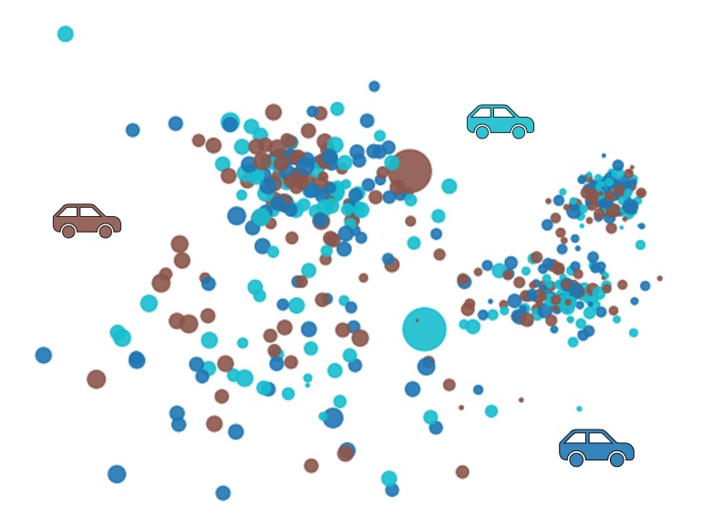
Figure 1: Random client assignments for the 3 Sales Representatives, Rep. Brown, Rep. Cyan and Rep. Blue.
Probably not optimal in terms of travel times.

We have been commissioned to do just that: (re)assign the 500 clients to the 3 salespersons’ portfolios in a way that reduces travel times.

Finally, some additional info which may or may not be relevant:

• Some clients are bigger than others in terms of generated revenue.
• The sky is blue.
• Sales representatives are incentivized through yearly bonuses to maximize the revenue generated by their portfolio.
• Tigers are awesome animals.

Easiest mission ever?

OK, let me reformulate our objective: we want to group clients into 3 geographical clusters such that clients in a given cluster are close to each other.

Sounds a lot like what K-Means is supposed to do! So let’s just convert the clients GPS coordinates into 2D cartesian coordinates, and run K-means with $K=3$. Aaaand, here is the result:

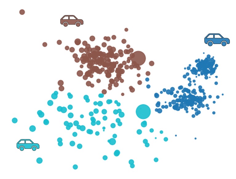
Figure 2: K-Means results. Travel times have been reduced. Good job everyone.

Boom, problem solved. Easiest money we’ve ever made.

💰💰💰

Mmmh? What’s that you say? Rep. Cyan is furious? Apparently, they’re saying the new assignment is really unfair, deprives them of clients, jeopardizes their annual bonus and are threatening to quit.

All right, all right, let’s take a quick look at the client distribution before we fly away to our well-deserved vacation.

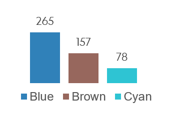
Figure 3: Clients repartition in clusters after K-Means optimization. Woops.

Woops, indeed! It looks like after we applied our brilliant optimization procedure, Rep. Cyan ended up with a meager 78 clients, whereas Rep. Blue generously got 265 clients. One of them sure is going to have an easier time generating high revenue from their clients portfolio.

Indeed, the implicit objective of our almighty K-Means is to minimize the (squared) distances within each cluster. Nowhere does it state that these clusters should have the same number of points. And indeed, there does not seem to be an option for that in the scikit-learn implementation we just so cleverly used.

Looks like our vacation will have to wait a little bit after all.

Under the hood of K-Means

So, K-Means does not do exactly what we want, but does not seem too far off either. Let’s take a closer look at what it does exactly, to see if there’s any chance we can find a quick fix to our problem.

Warning: here, I am not trying to explain how K-Means work to someone who has never heard of it. I am mostly (re)introducing the formalism behind it. If you need a more beginner-friendly introduction, you may want to look at other resources.

First, some formalism.

Assume that we have $N$ points in a $D$-dimensional space $\mathbf{X} = (\mathbf{x}_1, \mathbf{x}_2, \dots, \mathbf{x}_N)^\top \in \mathbb{R}^{N \times D}.$

We want to find two things:

• $\boldsymbol{K}$ centroids or cluster centers \(\mathbf{C} = (\mathbf{c}_1, \dots, \mathbf{c}_K)^\top \in \mathbb{R}^{K \times D}\)
• $\boldsymbol{N}$ assignments, which we can write as \(\mathbf{a} = (a_1, \dots, a_N)^\top \in \mathbb{N}^N\) that assign each \(\mathbf{x}_n\) to one of the $K$ centroids, such that \(a_n \in \{1, \dots, K\} ~~ \forall n\). Thus, $\mathbf{c}_{a_n}$ corresponds to the cluster center to which $\mathbf{x}_n$ is assigned.

The (sometimes implicit) objective of K-Means is to find $\mathbf{C}$ and $\mathbf{a}$ to minimize the inertia $J$ for a given dataset $\mathbf{X}$, defined as

\[\begin{equation} J_\mathbf{X}(\mathbf{C},\mathbf{a}) = \sum_{n=1}^{N} || \mathbf{x}_n - \mathbf{c}_{a_n} ||_2^2 \end{equation}\]

i.e. to solve the following problem:

\[\begin{equation} \underset{\mathbf{C},\mathbf{a}}{\text{minimize}} \quad J_\mathbf{X}(\mathbf{C},\mathbf{a}) \end{equation}\]

In other words, we try to find clusters so as to minimize the (squared) distances of each point \(\mathbf{x}_n\) to its corresponding cluster center $\mathbf{c}_{a_n}$.

As it turns out, in general the problem formulated in Equation (2) is NP-Complete, that is to say: not quite super easy to solve.

Thus, we typically try to find approximate solutions using a greedy heuristic: instead of trying to find both the cluster centers $\mathbf{C}$ and the assignments $\mathbf{a}$ at the same time as in Equation (2), we first assume that we already know the centroids $\mathbf{C}$, and minimize the inertia $J$ with respect to the assignments $\mathbf{a}$ only. Then, we assume that we already know the assignments $\mathbf{a}$, and minimize $J$ with respect to the centroids $\mathbf{C}$ only.

That is to say, we alternate between:

\[\begin{align*} \underset{\mathbf{a}}{\text{minimize}} \quad J_{\mathbf{X},\mathbf{C}}(\mathbf{a}) & \quad \quad \text{(E step)} \\ \underset{\mathbf{C}}{\text{minimize}} \quad J_{\mathbf{X},\mathbf{a}}(\mathbf{C}) & \quad \quad \text{(M step)} \\ \end{align*}\]

Why E step and M step?

K-Means can be seen as a special case of a more generic family of methods called Expectation-Maximization, consisting of alternating between an Expectation (E) step and a Maximization (M) step. It does not really matter for now though. I just kept these two names for the sake of consistency.

These two problems are actually pretty easy to solve. Indeed, we could prove that the solution to the E step is

\[\begin{equation} \text{(E step)}\quad \quad \underset{\mathbf{a}}{\text{minimize}} ~~ J_{\mathbf{X},\mathbf{C}}(\mathbf{a}) \quad \implies \quad a_n = \underset{k}{\text{argmin}} ~ ||\mathbf{x}_n - \mathbf{c}_k||_2^2 ~~ \forall n \end{equation}\]

i.e. we should assign each point to the closest cluster center (for each point $\mathbf{x}_n$, make the assignment $a_n$ correspond to the index $k$ of the cluster whose centroid $\mathbf{c}_k$ minimizes the (squared) distance to $\mathbf{x}_n$).

Similarly, the solution to the M step is

\[\begin{equation} \text{(M step)}\quad \quad \underset{\mathbf{C}}{\text{minimize}} ~~ J_{\mathbf{X},\mathbf{a}}(\mathbf{C}) \quad \implies \quad \mathbf{c}_k = \frac{1}{|\mathcal{X}_k|} \sum_{\mathbf{x} \in \mathcal{X}_k} \mathbf{x} ~~ \forall k \quad \text{with} \quad \mathcal{X}_k = \{\mathbf{x}_n ~|~ a_n = k\} \end{equation}\]

i.e. we should set each cluster as the mean of the points assigned to this cluster ($\mathcal{X}_k$ being defined as the set of points whose assignment $a_n$ is $k$).

All that is missing is a starting position to begin our alternating optimization. One possibility is to initialize centroids randomly.

This finally gives us the familiar K-Means algorithm:

1. Initialize $K$ centroids randomly
2. Assign each point to the cluster whose centroid is closest (E step)
3. Update centroids as the means of the corresponding assigned points (M step)
4. Repeat 2 and 3 until convergence

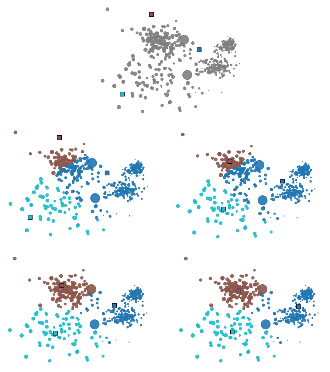
Figure 4: Illustration of K-Means in action: we first initialize $K$ centroids (top). Then we alternate between assigning each point to its closest centroid (E step, on the left), and updating each centroid as the means of the points assigned to it (M step, on the right).

About the NP-Completeness of K-Means

The fact that the inertia-minimization objective is NP-Complete naturally raises the question: is the approximate solution that we end up with using K-Means good enough? It turns out that, usually, yes. This series of blog posts provides some intuition about why this is the case.

“Right, right. I already (kinda) knew how K-Means works. It’s quite easy to understand from Figure 4 above. Why over-complicate things with all the previous obscure formalism?”

The point was to precisely define our objective, so that we can then (hopefully) solve the problem that we are actually interested in. For instance, we have seen that nowhere in the formulation of the K-Means objective or its resolution method is there any mention of the number of elements a cluster should have. Hence the unsuitable results that we obtained in the previous section.

What if we wanted to change that? Having balanced clusters is important in our use case, so let’s explicitly take that into account in the problem we want to solve. One way to express this is to modify the objective from Equation (2) to:

\[\begin{equation} \underset{\mathbf{C},\mathbf{a}}{\text{minimize}} ~~ % J_\mathcal{X}(\mathcal{C},\mathcal{A}) \sum_{n=1}^N || \mathbf{x}_n - \mathbf{c}_{a_n} ||_2^2 \quad \text{s.t.} ~ |\mathcal{X}_k| = \frac{N}{K} ~\forall k \end{equation}\]

i.e. we still want to find centroids $\mathbf{C}$ and assignments $\mathbf{a}$ that minimizes the (squared) distance from each point to its cluster center, with the added constraint that the sets of points $\mathcal{X}_k$ assigned to each cluster must all have the same number of points.

OK, we have defined the problem we are actually interested in.

Now, how do we solve it?

An alternative formulation of K-Means

I promise we’ll get there soon. For now, allow me to start by making some small changes to our K-Means problem formulation.

We will replace our $N$ integer variables \(a_n \in \{ 1, \dots, K\}\) with $N \times K$ dummy variables \(\alpha_{n,k} \in \{0, 1\}\), such that

\[\alpha_{n,k} = \begin{cases} 1 \quad \text{if} ~ a_n = k \\ 0 \quad \text{otherwise} \end{cases}\]

Let’s write \(\mathbf{A} = \begin{pmatrix} \alpha_{1,1} & \dots & \alpha_{1,K} \\ \vdots & \ddots & \vdots \\ \alpha_{N,1} & \dots & \alpha_{N,K} \\ \end{pmatrix} \in \{0,1\}^{N \times K}\) the set of all $N \times K$ binary variables $\alpha_{n,k}$.

The inertia $J$ can thus be rewritten as

\[J_\mathbf{X}(\mathbf{C},\mathbf{A}) = \sum_{n=1}^N \sum_{k=1}^K \alpha_{n,k} || \mathbf{x}_n - \mathbf{c}_{k} ||_2^2\]

This is the same problem as in Equation (2), so we still cannot solve it directly. But we can continue alternating between the previous E and M steps to find an approximate solution.

The M step (centroids update) can be rewritten as

\[\begin{equation} \text{(M step)}\quad \underset{\mathcal{C}}{\text{minimize}} ~ J_{\mathcal{X},\mathcal{\Alpha}}(\mathcal{C}) \quad \implies \quad \mathbf{c}_k = \frac{\sum_n \alpha_{n,k} \mathbf{x}_n}{\sum_n \alpha_{n,k}} ~~ \forall k \end{equation}\]

(because \(\sum_{\mathbf{x} \in \mathcal{X}_k} \mathbf{x} = \sum_n \alpha_{n,k} \mathbf{x}_n\) and \(|\mathcal{X}_k| = \sum_n \alpha_{n,k}\) in Equation 4)

And the E step (assignments update) objective can be rewritten as

\[\begin{align} \begin{split} \text{(E step)}\quad & \underset{\mathbf{A}}{\text{minimize}} ~ J_{\mathbf{X},\mathbf{C}}(\mathbf{A}) = \sum_{n,k} \alpha_{n,k} || \mathbf{x}_n - \mathbf{c}_{k} ||_2^2 \\ &\text{such that} \quad \sum_k \alpha_{n,k} = 1 ~ \forall n \\ % & \implies % \alpha_{n,k} = % \begin{cases} % 1 \quad \text{if} ~ k = \underset{i}{\text{argmin}} ~ ||\mathbf{x}_n - \mathbf{c}_i||_2^2 \\ % 0 \quad \text{otherwise} % \end{cases} % ~~ \forall n,k \end{split} \end{align}\]

The $N$ constraints $\sum_k \alpha_{n,k} = 1$ are necessary to ensure that for a given point $n$, exactly one $k$ is such that $\alpha_{n,k} = 1$, i.e. to ensure that each point is assigned to precisely one cluster. (Otherwise, simply choosing $\alpha_{n,k} = 0 ~ \forall n,k$ would be a trivial (and entirely useless) way to minimize the inertia $J$).

So far, the problem is exactly the same as in the previous part. However, there is something interesting about the reformulated E step objective: it can be viewed as an (integer) linear programming problem!

Linear programming

In general, linear programming problems are of this form:

\[\begin{align} \begin{split} \text{minimize} ~ & \sum_m x_m c_m \quad \text{w.r.t.} ~~ x_1, \dots, x_M \\ \text{such that} ~ & \sum_m x_m p_m \geq p_0 \\ & \sum_m x_m q_m \geq q_0 \\ & \quad \vdots \end{split} \end{align}\]

i.e. we want to find variables $x_m$s that minimize a linear combination, subject to a number of inequality constraints which are also linear combination of the variables $x_m$s.

Bonus exercise: write Equation (8) in matrix notation.

Without getting into too many details, there are efficient ways to solve linear programming problems, e.g. using Dantzig’s simplex algorithm. The fact that our variables $\alpha_{n,k}$s need to be binary/integers slightly complicates things, but again, practical solutions exist. For now, all we need to know is that some libraries such as pulp nicely provide easy-to-use solvers for this kind of problems.

In our specific case, we want to minimize \(\sum_{n,k} \alpha_{n,k} ||\mathbf{x}_n - \mathbf{c}_k||_2^2\) with respect to the $\alpha_{n,k}$s. The $\alpha_{n,k}$s play the role of the variables $x_m$ in Equation (8) above, and the $||\mathbf{x}_n - \mathbf{c}_k||_2^2$ play the role of the constants $c_m$.

The $\sum_k \alpha_{n,k} = 1 ~ \forall n$ in Equation (7) corresponds to $N$ constraints.

How do we go from $\sum_i x_i p_i \geq p_0$ to $\sum_k \alpha_{n,k} = 1$ ?

A first basic difference in the objective and constraints formulation is that in Equation (8), we have a sum $\sum_m$ over a single variable $m$, whereas in our specific problem (Equation 6), we have a double sum $\sum_n\sum_k$ over variables $n$ and $k$ — or equivalently a double sum $\sum_{n,k}$ over the tuple of variables $(n,k)$. However, it does not matter, as we could define a variable $m$ such that $m=1$ corresponds to $(n,k)=(1,1)$, $m=2$ to $(n,k)=(1,2)$ etc. up to $m=NK$ corresponding to $(n,k)=(N,K)$. So to simplify notations I am just going to keep the sum over $\sum_{n,k}$.

With that being said, how can we choose our $p_m$s (or equivalently $p_{n,k}$s) such that we end up with the $N$ constraints $\sum_k \alpha_{n,k} = 1 ~~ \forall n$?

For a given $n$, we can set

\[p_{i,k} = \begin{cases} 1 \quad \text{if } i=n \\ 0 \quad \text{otherwise} \end{cases}\]

as well as $p_0 = 1$.

This way, we end up with

\[\begin{equation} \sum_{i,k} \alpha_{i,k} p_{i,k} = \sum_k \alpha_{n,k} \geq 1 \end{equation}\]

Now, we add a second constraint with coefficients $q_m$s, defined such that $q_0 = -1$ and

\[q_{i,k} = \begin{cases} - 1 \quad \text{if } i=n \\ 0 \quad \text{otherwise} \end{cases}\]

This way, $\sum_{i,k} \alpha_{i,k} q_{i,k} = - \sum_k \alpha_{n,k} \geq -1$ i.e.

\[\begin{equation} \sum_k \alpha_{n,k} \leq 1 \end{equation}\]

The only possibility to enforce this constraint as well as the constraint from Equation (9) is to have $\sum_k \alpha_{n,k} = 1$.

We continue adding two such constraints for every $n$, and voilà! We have defined our objective and our constraints such that the E step optimization problem from K-Means has been reframed as a linear programming problem.

Note: most linear programming solvers actually enable to directly specify equality constraints instead, so in practice we generally only need to write a single constraint for each $n$.

Adding constraints

All right, let me recap: we already had a perfectly good way to (approximately) solve the K-Means objective. Now we have a new, more complicated way to solve it with intermediate linear programming problems. Why put ourselves through that?

Well, the neat thing is: we can now easily add further constraints in our intermediate linear programming problem!

In particular, recall from earlier (Equation 5) that our new objective, clustering with balance constraints, can for example be written as

\[\tag{11} % When <detail> is collapsed, equations inside are not rendered and so equation numbers are not incremented \underset{\mathbf{C},\mathbf{A}}{\text{minimize}} ~~ J_\mathbf{X}(\mathbf{C},\mathbf{A}) = \sum_{n,k} \alpha_{n,k} || \mathbf{x}_n - \mathbf{c}_{k} ||_2^2 \quad\quad \text{s.t.} ~ |\mathcal{X}_k| = N_k ~~\forall k\]

meaning that we want to minimize the inertia $J$ with the constraint that cluster $k$ contains exactly $N_k$ elements. Or, to provide our optimizer with a bit more room for maneuver, we may instead merely ask that each cluster contains at least $N_k$ elements instead, with a slightly smaller $N_k$, i.e. \(|\mathcal{X}_k| \geq N_k ~~\forall k\).

Similarly to K-Means, we don’t have a reliable way to directly solve this problem. But we may use the same alternating optimization trick:

\[\begin{align*} \text{(E step)} \quad\quad & \underset{\mathbf{A}}{\text{minimize}} \quad J_{\mathbf{X},\mathbf{C}}(\mathbf{A}) \quad \text{s.t.} ~ |\mathcal{X}_k| \geq N_k ~~\forall k \\ \text{(M step)} \quad\quad & \underset{\mathbf{C}}{\text{minimize}} \quad J_{\mathbf{X},\mathbf{A}}(\mathbf{C}) \quad \text{s.t.} ~ |\mathcal{X}_k| \geq N_k ~~\forall k \end{align*}\]

The solution to the M step is not affected by the $K$ constraints: whether or not they are satisfied, there is nothing we can do about that by changing the centroids’ locations. So we end up with the same solution as in Equation (6):

\[\mathbf{c}_k = \frac{\sum_n \alpha_{n,k} \mathbf{x}_n}{\sum_n \alpha_{n,k}} ~~ \forall k\]

Regarding the E step: since \(|\mathcal{X}_k|\), the size of cluster $k$, can be expressed as \(\sum_n \alpha_{n,k}\), the objective to the E step can now be written as

\[\tag{12} % When <detail> is collapsed, equations inside are not rendered and so equation numbers are not incremented \begin{align} \begin{split} \text{(E step)}\quad & \underset{\mathbf{A}}{\text{minimize}} \quad % ~ J_{\mathcal{X},\mathcal{C}}(\mathcal{\Alpha}) = \sum_{n,k} \alpha_{n,k} || \mathbf{x}_n - \mathbf{c}_{k} ||_2^2 \\ &\text{such that} \quad \sum_k \alpha_{n,k} = 1 \quad \forall n \\ &\phantom{\text{such that} \quad} \sum_n \alpha_{n,k} \geq N_k ~~ \forall k \\ \end{split} \end{align}\]

This is still a linear programming problem! Although we don’t have a direct generic formula for the corresponding optimal assignments $\alpha_{n,k}$ as in Equation (3), a linear programming solver can still easily find these optimal $\alpha_{n,k}$s for us.

So, we have a way to solve the E step and M step corresponding to our modified, constrained objective (Equation 11). Similarly to K-Means, we can alternate between the E and M step until we obtain an (approximate) solution to our global constrained optimization problem.

Here is our modified K-Means algorithm:

1. Initialize $K$ centroids randomly
2. Solve the E step: find the assignments $\alpha_{n,k}$s corresponding to our constrained objective from Equation (12) using a linear programming solver
3. Solve the M step: update centroids as the means of the corresponding assigned points
4. Repeat 2 and 3 until convergence

Bringing balance to the (sales)force

OK, sounds good in theory. Does it work in practice though?

Only one way to find out! Let’s implement this algorithm. Since we have a total of 500 points, let’s set $N_k=150 ~~\forall k$ so that each cluster contains at least 150 points. This should lead to approximately the same number of clients in each portfolio, while still leaving the solver with enough wiggle room to find a good geographical partitioning.

Aaaaand, we get…

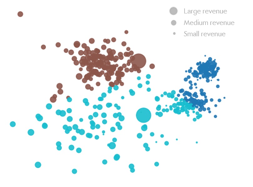
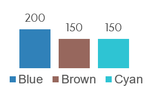
Figure 5. Left: geographical distribution of portfolios’ clients.
Right: number of clients within each cluster/portfolio.

Awesome! This is pretty much exactly what we wanted. Now we have good geographical clusters, while ensuring that these clusters are fairly balanced. (If this is not balanced enough for you, we also have the option to select a higher value of $N_k$, for instance $N_k=160$).

At last, we may take some rest!

The Rep.’s ire strikes back

Eh? What now?

Rep. Blue is angry? But they’re the one with the highest number of clients in their portfolio! How can they be unhappy? Something about the revenue you say? Fine, fine, let’s have a look…

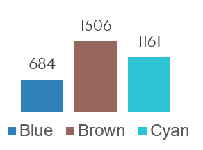
Figure 6: Total revenue for each cluster.

Oh, I see… Blue’s clients typically have low revenue (as is visible in Figure 5), so Blue’s portfolio has the lowest revenue despite having the highest number of clients.

Bummer. How can we make it so that the number of clients and the revenue are balanced?

That’s right, pretty much exactly the same way we solved our previous problem.

Assuming revenue for customer $n$ is given by $r_n$, total revenue for cluster $k$ is given by $\sum_n \alpha_{n,k} r_n$. Assuming we want revenue at least $R_k$ in cluster $k$, we get the constraints $\sum_n \alpha_{n,k} r_n \geq R_k ~\forall k$.

This is again linear with respect to the $\alpha_{n,k}$s. So we simply add the $K$ constraints $\sum_n \alpha_{n,k} r_n \geq R_k$ in the objective from Equation (11), which now becomes:

\[\begin{align*} \text{(E step)}\quad & \underset{\mathbf{A}}{\text{minimize}} \quad % ~ J_{\mathcal{X},\mathcal{C}}(\mathcal{\Alpha}) = \sum_{n,k} \alpha_{n,k} || \mathbf{x}_n - \mathbf{c}_{k} ||_2^2 \\ &\text{such that} \quad \sum_k \alpha_{n,k} = 1 \quad\quad~~ \forall n \\ &\phantom{\text{such that} \quad} \sum_n \alpha_{n,k} \geq N_k \quad\quad \forall k \\ &\phantom{\text{such that} \quad} \sum_n \alpha_{n,k} r_n \geq R_k \quad~ \forall k \end{align*}\]

We then repeat the other steps exactly as previously.

As an example, let’s say we want each cluster to have at least 30% of the total revenue $R = \sum_n r_n$. Then we can choose $R_k = 0.3 R ~\forall k$, which would be $R_k=1005$ in my example dataset.

This leads to:

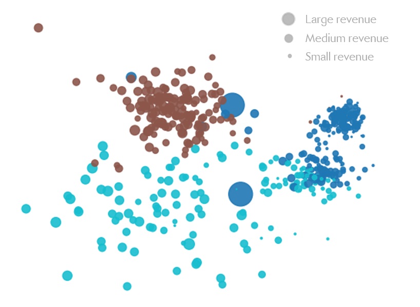
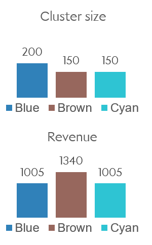
Figure 7. Left: geographical distribution of portfolios’ clients.
Right: number of clients and revenue for each cluster/portfolio.
This is getting easy.

Mmmh? Clients from cluster dudecomeonwhatnow are on average less friendly than clients from cluster whatever, and this is somehow really really important?

You guessed it: introduce friendliness score $f_n$ for client $n$, add $K$ constraints $\sum_n \alpha_{n,k} f_n \geq F_k$, and there you go.

Coffee tastes better at some clients’ than at others? Time for some koffee scores $k_n$ then.

No more jokes, only actually important constraints this time

All right, you may have guessed that the friendliness and coffee scores were not real constraints from the actual project. However, I would still like to address two further, slightly different constraints that were of considerable actual importance to this project.

The first one is related to special client-representative relationships. Let’s say Rep. Brown spent a considerable amount of time developing their two largest clients, Hugh and Hugo, and understandably does not want to give up this special relationship. This can be addressed by specifying

\[\begin{align*} \alpha_{\text{Hugh}, \text{Brown}} = 1 \\ \alpha_{\text{Hugo}, \text{Brown}} = 1 \end{align*}\]

Adding this along with the other constraints ensures that these two clients will be assigned to Rep. Brown. The rest of the parameters will be adjusted to take this constraint as well as the others into account, leading to e.g.:

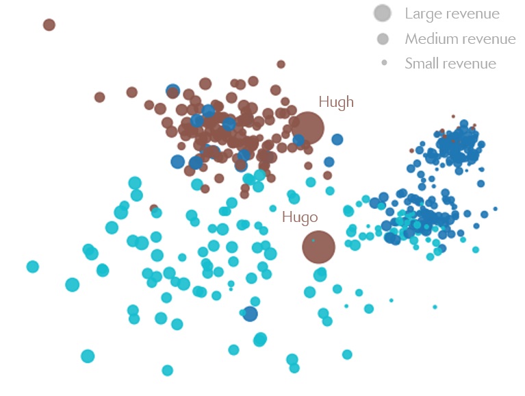
Figure 8: Hugh and Hugo belong to the Brown realm.

The second concern is related to the acceptable degree of change of a portfolio in a given year. Sales representatives may be OK with having some of their clients portfolio modified in exchange for improved travel times — provided this doesn’t jeopardize their yearly bonus of course. But changing almost all of their portfolio may still be too much, as getting to know a new client takes time.

Fortunately, this can again be addressed fairly easily using our framework. Writing $t_{n,k}$ the pre-existing binary assignments at time $t$ (before our optimization) such that

\[t_{n,k} = \begin{cases} 1 \quad \text{if client } n \text{ is currently in portfolio } k \\ 0 \quad \text{otherwise} \end{cases}\]

the constraint

\[\frac{1}{\sum_n t_{n,k}} \sum_n \alpha_{n,k} t_{n,k} \geq S_k\]

specifies that a ratio of at least $S_k$ of the assignments in cluster $k$ must stay the Same after the optimization. Since this is a linear combination of the $\alpha_{n,k}$s, we can add yet another set of $K$ constraints into our objective from Equation (12). Choosing e.g. $S_k = 70\% ~\forall k$ will thus ensure that at most 30% of existing clients are modified in any portfolio.

A word of caution

To recap, we have a really powerful framework: it can lead to balanced clusters, but as we have seen, it is much more expressive than that. For instance, we can also deliberately keep or create an unbalance for a subset of clusters, as e.g. a way to incentivize sales representatives to find new clients to add to their own portfolio — otherwise, finding new clients would not really be worth it if portfolios were completely rebalanced every year.

Yet, there are two things that I would like to emphasize regarding the constraints.

First, constraints expressed within this framework are hard constraints: no compromise can be found by having a constraint that is almost satisfied. This is entirely by design: doing otherwise would open a deep rabbit hole about the importance that each constraint should have with respect to every other, which is typically a terrible idea — and maybe a topic for a future blog post.

However, this has implications: most notably, some sets of constraints may not have any feasible solution. As an example, requiring that each of the 3 clusters contains at least 200 clients would obviously not work if the total number of clients is 500. But some more subtle combinations of constraints may also lead to less obviously intractable problems.

Example of an impossible combination of constraints

As a very quick example: let’s say the initial distribution of the 500 clients between clusters is $(100, 200, 200)$. We require that each cluster now has at least $150$ clients, and that each portfolio keeps at least $90\%$ of its existing clients. Taken separately, each of these two (sets of) constraints is feasible. But they cannot be satisfied at the same time: having 150 clients in cluster 1 would require that 50 clients are transferred to this portfolio; but the most we can take from clusters 2 and 3 is 10% of the existing clients, which thus cannot be more than 20 + 20 = 40 clients.

Second, even under the assumption that the constraints do not lead to an intractable problem, adding new constraints typically comes at a cost regarding the quality of the geographical clustering. This is starting to be visible in Figure 8, where we can see that the homogeneity of the clusters is starting to suffer from all the constraints that were added.

Measuring the inertia after our successive additions of constraints, this is what we get:

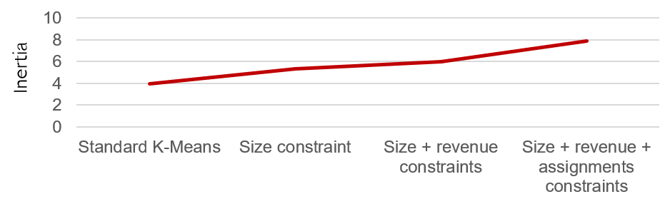
Figure 9: Inertia with no constraint, a single size constraint, then more and more constraints.

So in general, one should be wary about adding too many constraints, and try to limit oneself to those that are really necessary.

Final words

OK, that’s about it.

A couple of words regarding the actual project: as you may have guessed, it was not limited to just 500 clients in one territory. The idea was more to create a general framework that would enable optimizing dozens of territories of varying sizes for different subsidiaries of my client. But the overall idea was generally the same. To be honest, this is work I am reasonably proud of.

The method described here was implemented in Python, using pulp as the linear optimization solver. I have not yet cleaned or published the code I used to solve the problems of this blog post and to generate the corresponding visuals, but I may consider doing so in the future. Let me know if this might be of interest to you.

All right, thanks for reading, and see you next time!

Don’t want to miss the next post? You can follow me on Twitter!